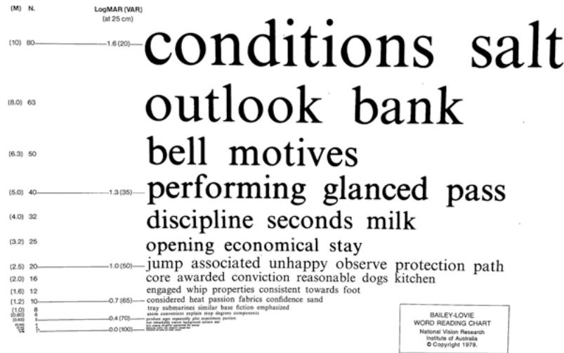
Fig. 1.3 The Bailey– Lovie word reading chart
1.2.2 Contrast Sensitivity Tools
Contrast sensitivity testing was first demonstrated in 1978 using Arden gratings and consisted of varying spatial frequencies and contrast levels. Based on similar principles, the functional acuity contrast test, first described by Arthur Ginsburg, consists of sine wave gratings of varying spatial frequencies and contrast levels [16] . The most popularly known contrast sensitivity test, the Pelli–Robson contrast sensitivity chart, was developed by DG Pelli, JG Robson, and AJ Wilkins; they published the design of this chart in 1988 [17] . In the Pelli–Robson contrast sensitivity chart (Fig. 1.4), English letters in triplets with fixed spatial frequency (i.e., constant size) vary in contrast levels. The optotype size subtends 2.8° at 1 m (~20/672) (appropriate for patients with visual impairment), which is equivalent to 20/224 at 3 m (~2.67 CPD [cycles per degree]) (recommended testing distance). The logCS was comparable at these two testing distances [18]. This chart measures contrast sensitivity from 0.00 to 2.25 logCS range. The higher the logCS, the better the contrast sensitivity. The chart has good repeatability of ±0.15 log units in young and older adults [19].
In addition, there are several commercially available contrast sensitivity tools using various targets such as pictures (hiding Heidi contrast sensitivity test) (Fig. 1.5, left), gratings contrast sensitivity test) [21], and circles (spot (Cambridge low-contrast gratings, Ohio contrast checks) [22]. cards [20] (Fig. 1.5, right), letters (Mars letter
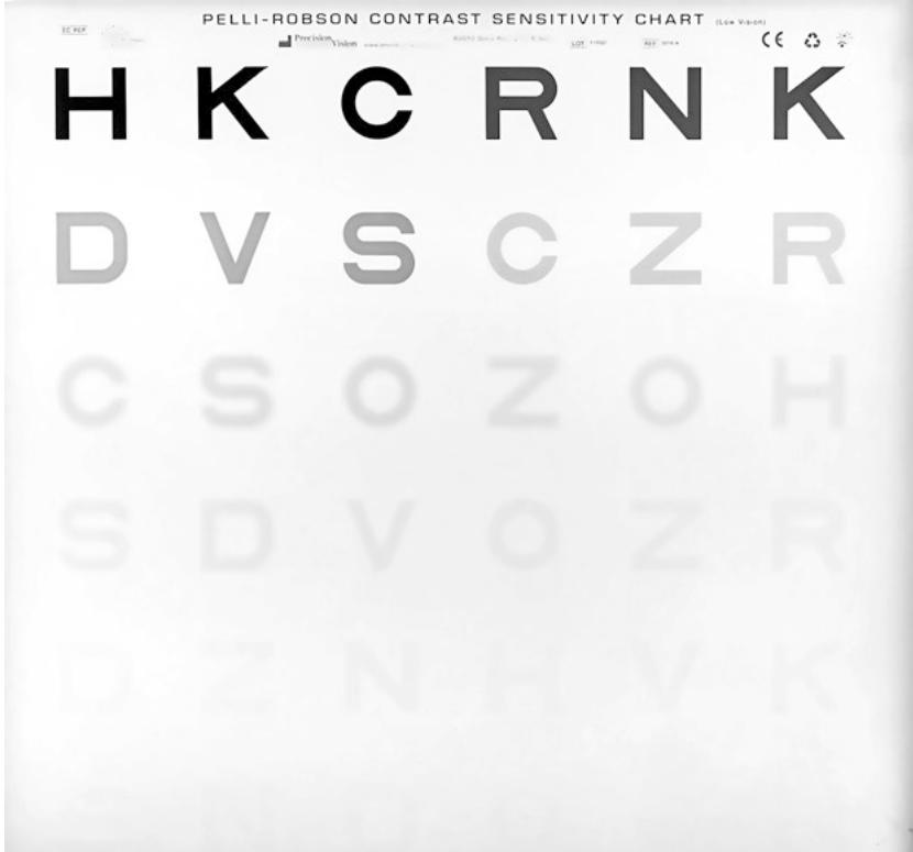
Fig. 1.4 The Pelli–Robson contrast sensitivity chart placed in a lightbox

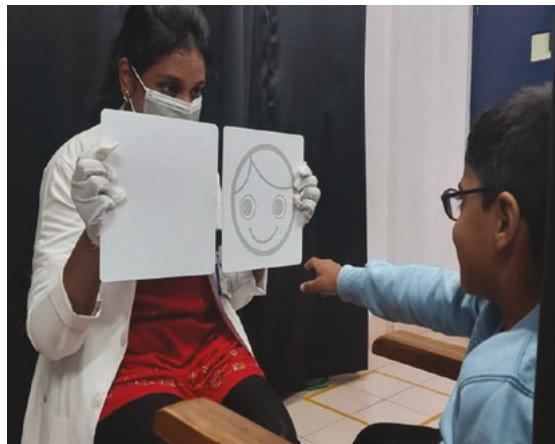
Fig. 1.5 Contrast sensitivity assessment using (left) the hiding Heidi low-contrast face test and (right) Ohio contrast cards
1.3 Underlying Concept
1.3.1 Distance Visual Acuity
Visual acuity is the resolution capacity of an eye. The resolution capacity is the smallest gap an eye can detect between two objects. This gap would subtend an angle at the nodal point of the eye. Therefore, the smallest angle resolved by the eye is its visual acuity (Fig. 1.6). Any angle or separation smaller than this would result in a single blurred object instead of two distinct objects. The smallest visual angle a human eye could resolve is about 1′ (1 min of arc) (see Box 1.1) [23].
As seen in Fig. 1.6, two black lines with a white separation will require a minimum of 3 photoreceptors to resolve it. One photoreceptor detects one dark line, another photoreceptor detects the white space, and a third adjacent photoreceptor detects the other dark line. If we consider one dark line and the white space as one cycle, then two dark lines separated by a white space will have 1.5 cycles. Therefore, to resolve 1.5 cycles, three photoreceptors (i.e.,) double the cycles are required. This limit of how many minimum photoreceptors are required to resolve an object is called the Nyquist limit. This is a borrowed concept from signal processing in electronics. If we consider the eye a device to capture and process light signals, the minimum number of photoreceptors required will be twice the spatial frequency (cycles per degree or CPD). Hence, to resolve 10 cycles, 20 photoreceptors are needed. Given this, and with the anatomical limi-
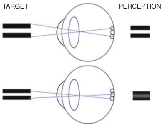
Fig. 1.6 An illustration of the minimum angle of resolu tion (MAR) to discern a black-and-white grating. A mini mum of three photoreceptors are required to see the grating target (top panel). If the grating subtends a smaller angle than the MAR, then a blurred blob of the grating is seen, which makes it indiscernible (lower panel)